All too often, we hear that businesses want to do more with their customer data. They want to be data-informed, they want to provide better customer experiences, and—most of all—they just want to understand their customers.
Getting there isn’t easy. Not only do you need to collect and store the data, you also need to identify the useful pieces and act on the insights.
At Segment, we’ve helped thousands of businesses walk the path toward becoming more data-informed. One successful technique we’ve seen time and time again is establishing a working data lake.
A data lake is a centralized repository that stores both structured and unstructured data and allows you to store massive amounts of data in a flexible, cost effective storage layer. Data lakes have become increasingly popular both because businesses have more data than ever before, and it’s never been cheaper and easier to collect and store it all.
In this post, we’ll dive into the different layers to consider when working with a data lake.
-
We’ll start with an object store, such as S3 or Google Cloud Storage, as a cheap and reliable storage layer.
-
A central piece is a metadata store, such as the AWS Glue Catalog, which connects all the metadata (its format, location, etc.) with your tools.
-
Finally, you can take advantage of a transformation layer on top, such as EMR, to run aggregations, write to new tables, or otherwise transform your data.
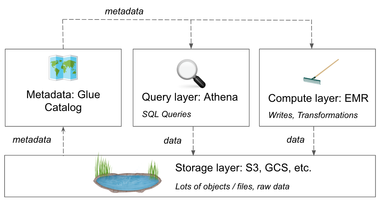
As heavy users of all of these tools in AWS, we’ll share some examples, tips, and recommendations for customer data in the AWS ecosystem. These same concepts also apply to other clouds and beyond.
Storage Layer: S3
If you take one idea away from this blog post, let it be this: store a raw copy of your data in S3.
It’s cheap, scalable, incredibly reliable, and plays nicely with the other tools in the AWS ecosystem. It’s very likely your entire storage bill for S3 will cost you less than a hundred dollars per month. If we look across our entire customer base, less than 1% of our customers have an S3 bill over $100/month for data collected by Segment.
That said, the simplicity of S3 can be a double-edged sword. While S3 is a great place to keep all of your data, it often requires a lot of work to collect the data, load it, and actually get to the insights you’re looking for.
There are three important factors to keep in mind when collecting and storing data on S3:
-
encoding – data files can be encoded any number of ways (CSV, JSON, Parquet, ORC), and each one can have big performance implications.
-
batch size – file size has important ramifications, both for your uploading strategy (and data freshness) and for your query times.
-
partition scheme – partitions refers to the ‘hierarchy’ for data, and the way your data is partitioned or structured can impact search performance.
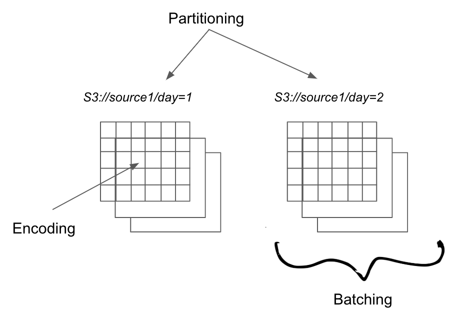
Structuring data within your data lake
We’ll discuss each of these in a bit more depth, but first it’s worth understanding how data first enters your data lake.
There are a number of ways to get data into S3, such as uploading via the S3 UI or CLI. But if you’re talking customer data, it’s easy to start delivering your data to S3 via the Segment platform. The Segment platform provides the infrastructure to collect, clean, and control your first party customer data and send exactly what you need to all the tools you need it in.
Encoding
The encoding of your files has a significant impact on the performance of your queries and data analysis. For large workloads, you’ll want to use a binary format like Parquet or ORC (we’re beginning to support these natively. If you’d like beta access, please get in touch!).
To understand why, consider what a machine has to do to read JSON vs Parquet.
When looking at JSON, the data looks something like this:
{ 'userId': 'user-1', 'name': 'Lauren', 'company': 'Segment' } { 'userId': 'user-2', 'name': 'Parsa', 'company': 'Segment } { 'userId': 'user-3', 'company': 'Microsoft', 'name': 'Satya' } { 'userId': 'user-4', 'name': 'Elon', 'company': 'Tesla' }
Here, we must parse not only the whole message, but each key individually, and each value. Because each JSON object might have a different schema (and is totally unordered), we have to do roughly the same work for each row.
Additionally, even if we are just picking out companies, or names, we have to parse all of our data. There’s no ‘shortcut’ where we can jump to the middle of a given row.
Contrast that with Parquet, and we see a much different schema. In Parquet, we’ve pre-defined the schema ahead of time, and we end up storing columns of data together. Below is an example of the previous JSON document transformed in Parquet format. You can see the users are stored together on the right, as they are all in the same column.

See users stored together on the right
A reader doesn’t have to parse out and keep a complicated in-memory representation of the object, nor does it have to read entire lines to pick out one field. Instead it can quickly jump to the section of the files it needs and parse out the relevant columns.
Instead of just taking my word for it, below are a few concrete benchmarks which query both JSON and Parquet.
In each of the four scenarios, we can see big gains from using Parquet.
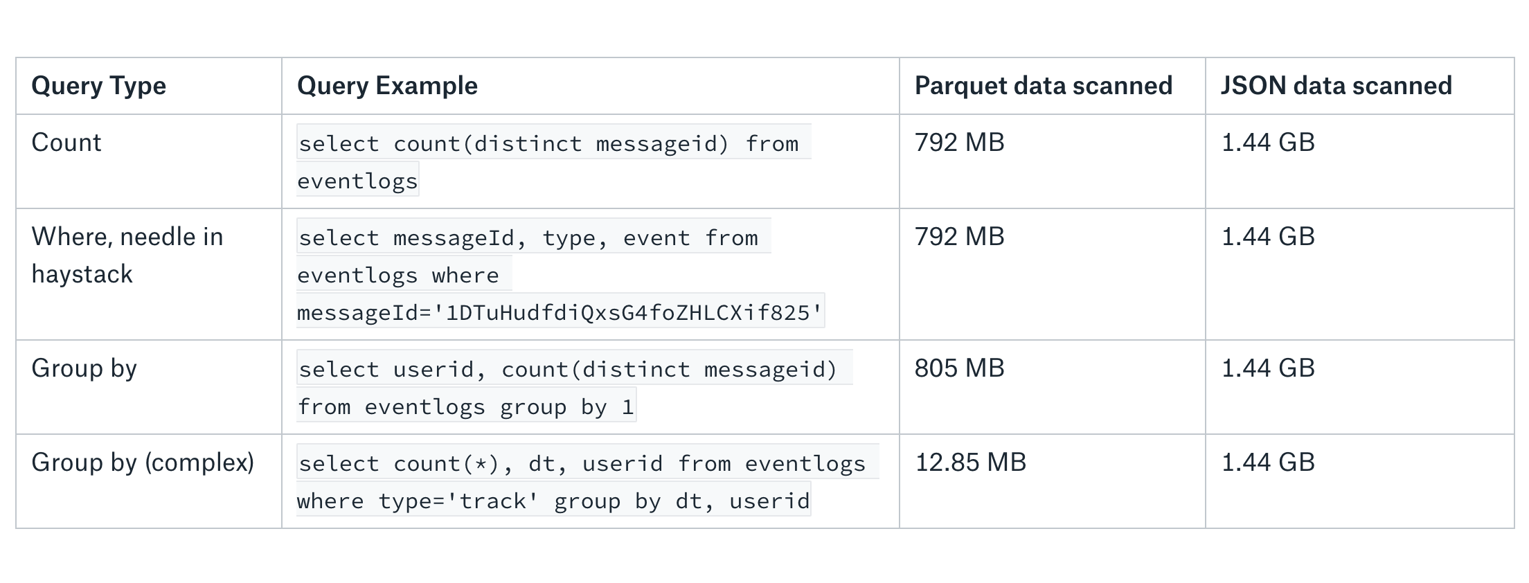
As you can see, the data we need to query in each instance is limited for Parquet. For JSON, we need to query the full body of each JSON event every time.
Batch Size
Batch size, or the amount of data in each file, is tricky to tune. Having too large of a batch means that you will have to re-upload or re-process a lot of data in the case of a hiccup or machine failure. Having a bunch of files which are too small means that your query times will likely be much longer.
Batch size is also tied to encoding, which we discussed above. Certain formats like Parquet and ORC are ‘splittable’, where files can be split and re-combined at runtime. JSON and CSV can be splittable under certain conditions, but typically cannot be split for faster processing.
Generally, we try and target files with sizes ranging from 256 MB to 1 GB. We find this gives the best overall performance mix.
Partitioning
When you start to have more than 1GB of data in each batch, it’s important to think about how a data set is split, or partitioned. Each partition contains only a subset of the data. This increases performance by reducing the amount of data that must be scanned when querying with a tool like Athena or processing data with EMR. For example, a common way to partition data is by date.
Querying
Finally, it’s worth understanding that just having your data in S3 doesn’t really directly help you do any of the things we talked about at the beginning of the post. It’s like having a hard drive, but no CPU.
There are many ways to examine this data — you could download it all, write some code, or try loading it into some other database.
But the easiest is just to write SQL. That’s where Athena comes in.
Query Layer: Athena 🔎
Once you’ve got your data into S3, the best way to start exploring what you’ve collected is through Athena.
Athena is a query engine managed by AWS that allows you to use SQL to query any data you have in S3, and works with most of the common file formats for structured data such as Parquet, JSON, CSV, etc.
In order to get started with Athena, you just need to provide the location of the data, its format, and the specific pieces you care about. Segment events in particular have a specific format, which we can leverage when creating tables for easier analysis.
Setup
Below is an example to set up a table schema in Athena, which we’ll use to look at how many messages we’ve received by type:
CREATE EXTERNAL TABLE IF NOT EXISTS segment_logs.eventlogs ( anonymousid string , # pick columns you care about! context map<string,string> , # using a map for nested JSON messageid string , timestamp Timestamp , type string , userid string , traits map<string,string> , event string ) PARTITIONED BY (sourceid string) # partition by the axes you expect to query often, sourceid here is associated with each source of data ROW FORMAT SERDE 'org.apache.hive.hcatalog.data.JsonSerDe' LOCATION 's3://your-s3-bucket/segment-logs' # location of your data in S3
In addition to creating the table, you will need to add the specific partitions:
ALTER TABLE eventlogs ADD PARTITION (sourceid='source1') LOCATION 's3://your-s3-bucket/segment-logs/sourceid=source1/' # sourceid here is associated with each source of data PARTITION (sourceid='source2') LOCATION 's3://your-s3-bucket/segment-logs/sourceid=source2/' PARTITION (sourceid='source3') LOCATION 's3://your-s3-bucket/segment-logs/sourceid=source3/' PARTITION (sourceid='source4') LOCATION 's3://your-s3-bucket/segment-logs/sourceid=source4/'
There are many ways to partition your data. Here, we’ve partitioned by source for each customer. This works for us when we’re looking at a specific customer, but if you’re looking across all customers over time, you may want to partition by date instead.
Query time!
Let’s answer a simple question from the table above. Let’s say we want to know how many messages of each type we saw for a given data source in the past day - we can simply run some SQL to find out from the table we just created in Athena:
select type, count(messageid) from eventlogs where sourceid='source1' and date_trunc('day', timestamp) = current_date group by 1 order by 2 desc
For all queries, the cost of Athena is tightly related to how you partition your data and its format. It is also driven by how much data is scanned ($5 per TB).
When scanning JSON, you will be scanning the entire record every time due to how it’s structured (see above for an example). Alternatively, you can set up Parquet for a subset of your data containing only the columns you care about, which is great for limiting your table scans and therefore limiting cost. This is also why Parquet can be so much faster—it has direct access to specific columns without scanning the full JSON.
Metadata: AWS Glue 🗺
Staying current
One challenge with Athena is keeping your tables up to date as you add new data to S3. Athena doesn’t know where your new data is stored, so you need to either update or create new tables, similar to the query above, in order to point Athena in the right direction. Luckily there are tools to help manage your schema and keep the tables up to date.
The AWS Glue Catalog is a central location in which to store and populate table metadata across all your tools in AWS, including Athena. You can populate the catalog either using out of the box crawlers to scan your data, or directly populate the catalog via the Glue API or via Hive. You can see how these all fit together in the diagram below.
Once this is populated with your metadata, Athena and EMR can reference the Glue Catalog for the location, type, and more when querying or otherwise accessing data in S3.
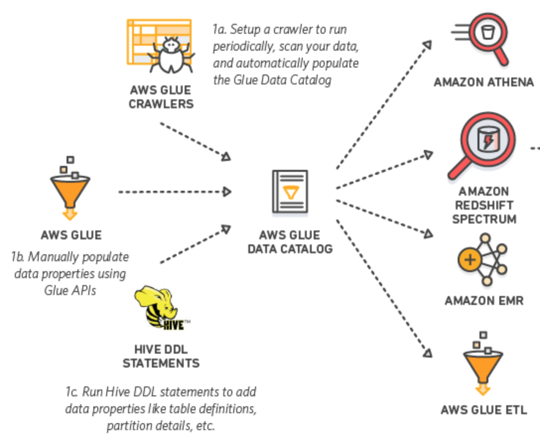
From: https://docs.aws.amazon.com/athena/latest/ug/glue-athena.html
Compute Layer: EMR
Moving beyond one-off queries and exploratory analysis, if you want to modify or transform your data, a tool like EMR (Elastic Map Reduce) gives you the power to not only read data but transform it and write into new tables. You may need to write if you want to transform the format of your data from JSON to Parquet, or if you want aggregate % of users completed the signup flow the past month and write it to another table for future use.
Operating EMR
EMR provides managed Hadoop on top of EC2 (AWS’s standard compute instances). Some code and config is required - internally we use Spark and Hive heavily on top of EMR. Hive provides a SQL interface over your data and Spark is a data processing framework that supports many different languages such as Python, Scala, and Java. We’ll walk through an example and more in-depth explanation of each below.
Pattern-wise, managing data with EMR is similar to how Athena operates. You need to tell it where your data is and its format. You can do this each time you need to run a job or take advantage of a central metastore like the AWS Glue Catalog mentioned earlier.
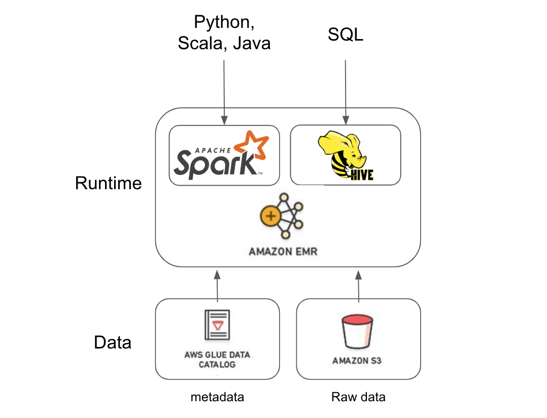
Building on our earlier example, let’s use EMR to find out how many messages of each type we received not only over the past day, but for every day over the past year. This requires going through way more data than we did with Athena, which means we should make a few optimizations to help speed this up.
Data Pre-processing
The first optimization we should make is to transform our data from JSON to Parquet. This will allow us to significantly cut down on the amount of data we need to scan for the final query, as shown previously!
For this JSON to Parquet file format transformation, we’ll want to use Hive, then turn to Spark for the aggregation steps.
Hive is a data warehousing system with a SQL interface for processing large amounts of data and has been around since 2010. Hive really shines when you need to do heavy reads and writes on a ton of data at once, which is exactly what we need when converting all our historical data from JSON into Parquet.
Below is an example of how we would execute this JSON to Parquet transformation.
First, we create the destination table with the final Parquet format we want, which we can do via Hive.
CREATE EXTERNAL TABLE `test_parquet`( anonymousid string , context map<string,string> , messageid string , timestamp Timestamp , type string , userid string , traits map<string,string> , event string ) PARTITIONED BY (dt string) -- dt will be the prefix on your output files, i.e. s3://your-data-lake/parquet/dt=1432432423/object1.gz STORED AS PARQUET -- specify the format you want here location 's3://your-data-lake/parquet/';
Then we simply need to read from the original JSON table and insert into the newly created Parquet table:
INSERT INTO test_parquet partition (dt) SELECT anonymousid, context, messageId, `timestamp`, `type`, userid, traits, event FROM test_json;
To actually run this step, we will need to create an EMR job to put some compute behind it. You can do this, by submitting a job to EMR via the UI:
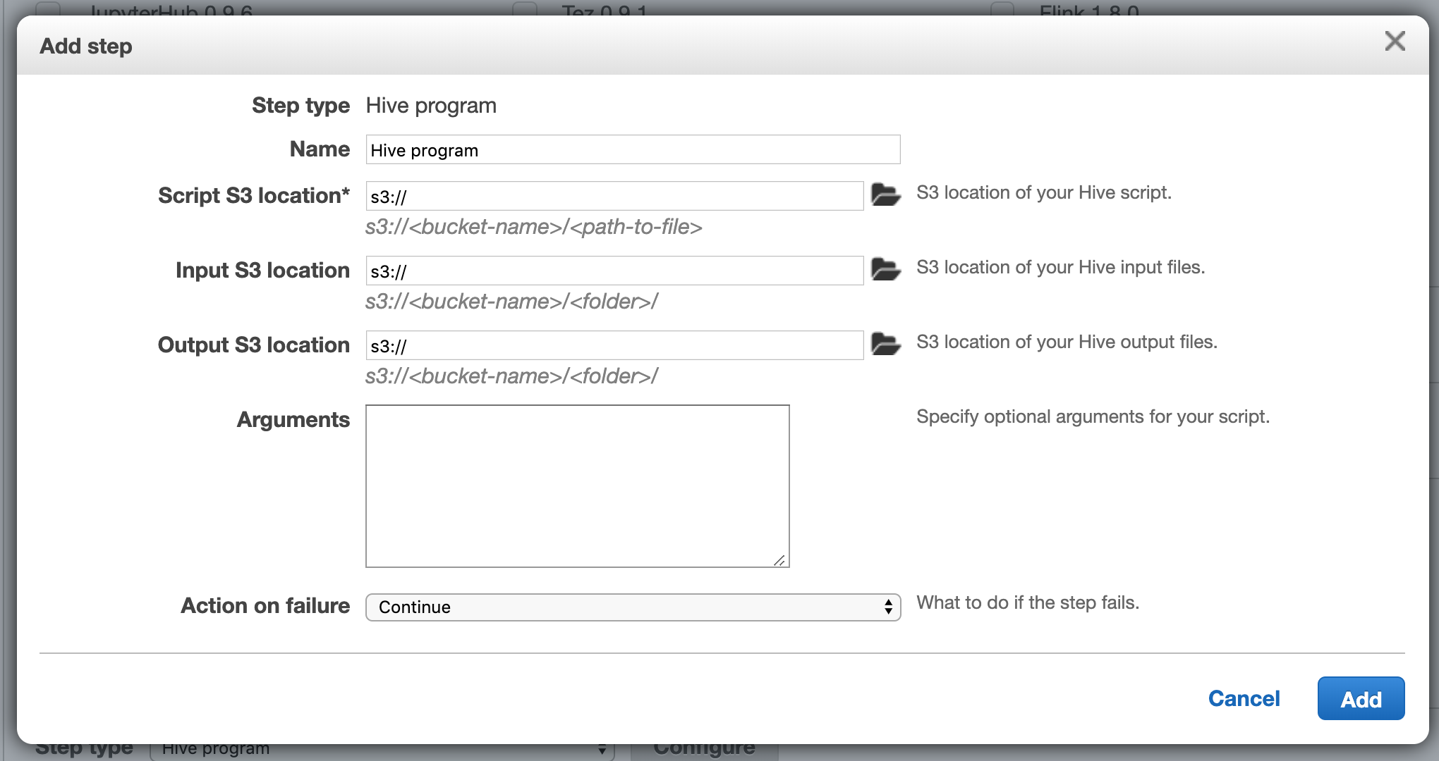
Or, by submitting a job via the CLI:
# EMR CLI example job, with lots of config! aws emr add-steps --cluster-id j-xxxxx --steps Type=spark, Name=SparkWordCountApp, Args=[ --deploy-mode,cluster,--master,yarn,--conf,spark.yarn.submit.waitAppCompletion=false,--num-executors,5,--executor-cores,5,--executor-memory,20g,s3://codelocation/wordcount.py,s3://inputbucket/input.txt,s3://outputbucket/], ActionOnFailure=CONTINUE
Aggregations
Now that we have our data in Parquet format, we can take advantage of Spark to sum how many messages of each type we received and write the results into a final table for future reference.
Spark is useful to run computations or aggregations over your data. It supports languages beyond SQL such as Python, R, Scala, Java, etc. which have more complex logic and libraries available. It also has in memory caching, so intermediate data doesn’t write to disk.
Below is a Python example of a Spark job to do this aggregation of messageid by type.
from datetime import datetime, timezone, timedelta from pyspark.sql.functions import col, when, count, desc # S3 buckets for reading Segment logs and writing aggregation output read_bucket_prefix = 's3://bizops-data-lake/segment-logs/source1' write_bucket_prefix = "s3://bizops-data-lake-development/tmp/segment-logs-source1"
# get datestamp for prior year today = datetime.now() last_year_partition = datetime.strftime(today - timedelta(years=today.weekday(), years=1), '%Y-%m-%d') last_year_ds = datetime.strptime(last_year_partition, '%Y-%m-%d') """ obtain all logs partitions of the year sample filenames: [ 's3://bizops-data-lake/segment-logs/source1/1558915200000/', 's3://bizops-data-lake/segment-logs/source1/1559001600000/', 's3://bizops-data-lake/segment-logs/source1/1559088000000/', ... ] """ read_partitions = [] for day in range(365): next_ds = last_year_ds + timedelta(days=day) ts_partition = int(1000*next_ds.replace(tzinfo=timezone.utc).timestamp()) read_year_partitions.append("{}/{}/".format(read_bucket_prefix, ts_partition))
# bucket partition for aggregation output # sample 's3://bizops-data-lake-development/tmp/segment-logs-source1/week_ds=2019-05-27/' write_year_ds = "{}/week_start_ds={}/".format(write_bucket_prefix, last_year_partition)
# read logs of last year, from pre-processing step. Faster with parquet! df = spark.read.parquet(read_year_partitions)
# aggregate by message type agg_df = df.select("type", "messageid").groupBy("type").agg( count(messageid).alias("message_count"), )
# writing Spark output dataframe to final S3 bucket in parquet format agg_df.write.parquet(path=write_year_ds, compression='snappy', mode='overwrite')
It is this last step, agg_df.write.parquet, that takes the updated aggregations that are stored in an intermediate format, a DataFrame, and writes these aggregations to a new bucket in Parquet format.
Conclusion
All in, there is a robust ecosystem of tools that are available to get value out of the large amounts of data that can be amassed in a data lake.
It all starts with getting your data into S3. This gives you an incredibly cheap, reliable place to store all your data.
From S3, it’s then easy to query your data with Athena. Athena is perfect for exploratory analysis, with a simple UI that allows you to write SQL queries against any of the data you have in S3. Parquet can help cut down on the amount of data you need to query and save on costs!
AWS Glue makes querying your S3 data even easier, as it serves as the central metastore for what data is where. It is already integrated with both Athena and EMR, and has convenient crawlers that can help map out your data types and locations.
Finally, EMR helps take your data lake to the next level, with the ability to transform, aggregate, and create new rollups of your data with the flexibility of Spark, Hive, and more. It can be more complex to manage, but its data manipulation capabilities are second to none.
At Segment, we help enable seamless integration with these same systems. Our S3 destination enables customers to have a fresh copy of all their customer and event data in their own AWS accounts.
We’re working on making this even easier by expanding the file format options, as well as integrating with the AWS Glue metastore, so you always have an up to date schema to keep up to date with your latest data. Drop us a line if you want to be part of the beta!
Special thanks to Parsa Shabani, Calvin French-Owen, and Udit Mehta

The State of Personalization 2023
Our annual look at how attitudes, preferences, and experiences with personalization have evolved over the past year.